SLAM
As part of my Masters of robotics program at Northwestern University I had 10 weeks to implement a SLAM (Simultaneous Localization And Mapping) algorithm from scratch. SLAM involves using sensors onboard a vehicle to detect landmarks to create a map of the surroundings and make traversing the environment easier.
This implementation was meant to simulate a turtlebot3 burger which is a differential drive robot with a rotating lidar sensor on the top of the robot.
Table of Contents
Demo Video
The video below shows a successful implementation of the SLAM algorithm using a Kalman Filter. There are three modeled turtlebots that represent the following:
Red: Simulated robot with collision and source of LiDAR measurements
Blue: Estimated location of the red robot using only odometry
Green: Estimated location of the red robot using both odometry and the SLAM algorithm
Video demonstration of the functional simulated SLAM algorithm
This implementation is successful because the green SLAM estimation robot follows the red robot closely even when the blue odometry estimation drifts. The blue robot can drift from the red “real” robot for two reasons: noise in the wheel rotations, and the inability to account for collisions with odometry. Noise has been added to the simulation where if a wheel is commanded to move 1 radian it may only move 0.98 radians to more accurately simulate a real robot. Since odometry cannot account for collisions with obstacles, the blue robot would drive through obstacles whereas the red robot would stop at them.
Odometry
The motors on the turtlebot3 burger have encoders that can tell to what extent each wheel has rotated. By using that data and integrating the wheel rotation over time an estimation of the location of the simulated robot can be calculated. The estimated location is then fed into the Kalman Filter. Below is a photo demonstrating that the blue robot can follow the red robot very closely if no obstacles are encountered, but the blue robot drifts significantly if an obstacle is hit.
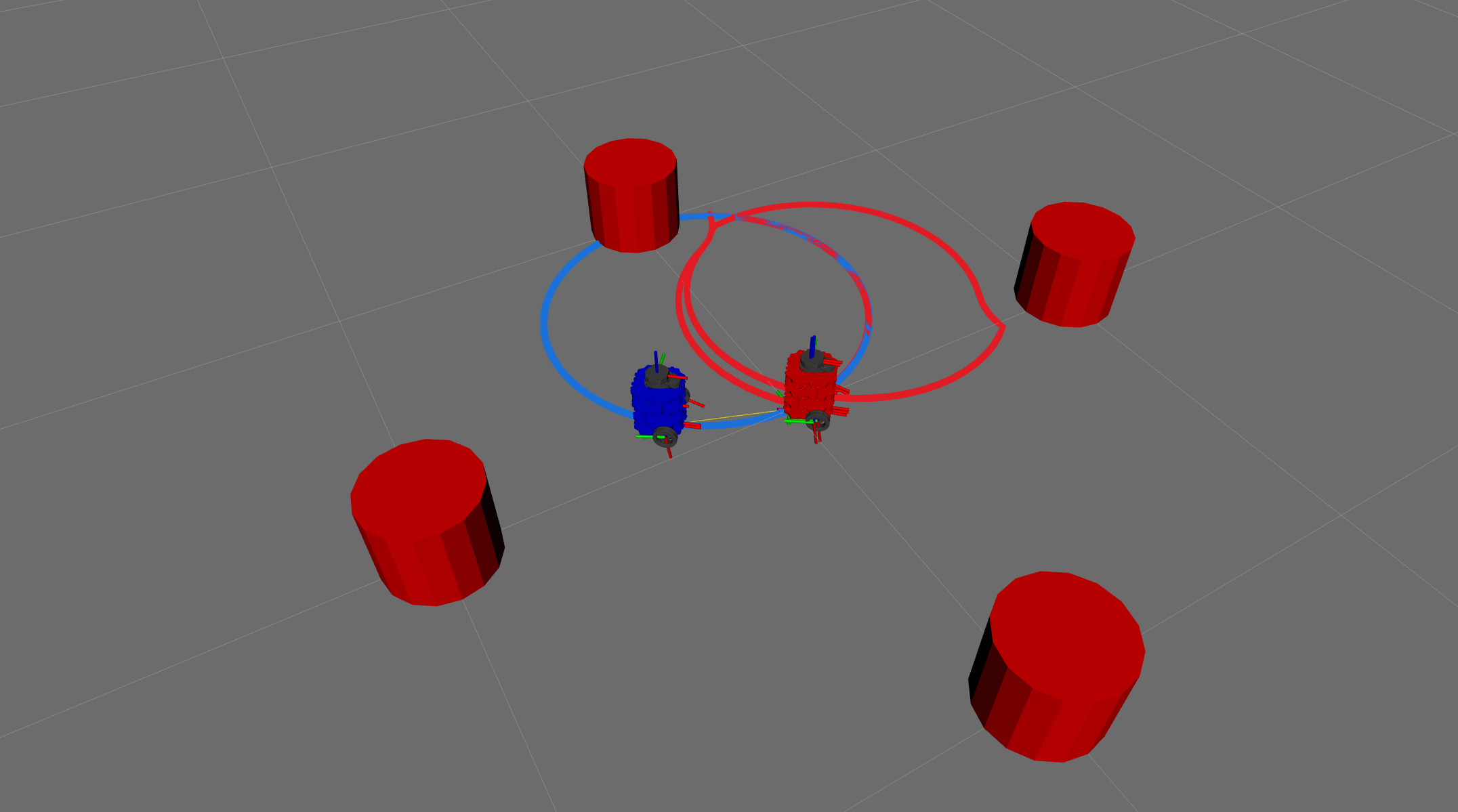
The above image shows the robots’ paths in their respective colors. This shows the red robot colliding with obstacles and eventually driving around them while the blue robot drives through them.
Simulated LiDAR
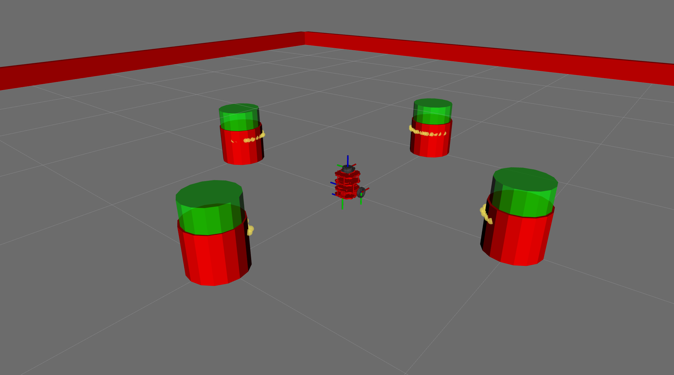
The turtlebot3 burger has a rotating LiDAR sensor onboard that obtains distance measurements around the robot multiple times a second. Below is a picture showing yellow orbs on the obstacles in the arena where the LiDAR beams hit the obstacles’ surfaces. These measurements are the second input into the Kalman Filter that localizes the robot in the space.
Kalman Filter
Using the odometry data, the data from the LiDAR sensor, and the previous estimation of the red robot’s location, a location estimate can be made at regular intervals. These estimates become increasingly accurate over time due to weights put on each source of data that change as more data is collected. In a Kalman Filter, weights are analogous to levels of trust in a specific source of data where an increasing weight means that the model thinks that source of data is more accurate. Starting off, the odometry has a high weight that begins to lower as the weight for the LiDAR rises with increasing measurements.